
May 6, 2025
Nuclear Magnetic Resonance is a key experimental method in condensed matter and biochemistry, and the basis of MRI technology. In this study, pulsed NMR techniques were used to generate spin echo signals from which relaxation constants were calculated. Due to signal noise limitations, methods robust against noise were developed. From these methods, the magnetic moment of the proton was measured, \(\mu_p = 1.416e-26 \pm 1.74e-29\) J/T. Further, relaxation constants for glycerin, water, and Copper Sulfate from \(10^{17}\) to \(10^{20}\) ions/mL were measured, revealing insights into the dependence of relaxation on viscosity and dissolved ion concentration.
Nuclear magnetic resonance is a common experimental tool used to study the internal structure of matter at a molecular level. The method is used in fields ranging from condensed matter physics and the study of strongly correlated electron systems, to biochemistry, where it can determine the structure of biological macromolecules. Nuclear magnetic resonance is also the fundamental mechanism behind magnetic resonance imaging, or MRI’s, in clinical settings.
In principle, nuclear magnetic resonance (NMR) uses the interaction between nuclear spins and applied magnetic fields. In a classic NMR experiment, a material is placed in a strong magnetic field \(H_0\). Since the spins of the nuclei in the material produce magnetic moments, \(\vec{\mu_p} = \gamma\vec{S}\), they will feel a torque from an applied magnetic field, given by: \[\vec{\tau} = \vec{\mu_p}\times\vec{H}\] Owing to the common result in quantum mechanics, the spins will precess about the magnetic field vector, say \(H_0\hat{z}\), due to their uncertainty in the two other spatial directions. The frequency of the spins precession about the field \(H_0\) is referred to as the Larmor frequency. Next, a much smaller magnetic field, \(H_1\), is applied perpendicular to \(H_0\) (say in the \(\hat{x}\) direction), which oscillates in time: \(\vec{H_1} = H_1\cos(\omega_1t)\hat{x}\). A common trick to elicit the effect of adding \(H_1\) is to convert to a rotating coordinate system, where the effective field felt by the spins becomes\(^{[1]}\): \[\vec{H_{eff}} = (H_0 - \frac{\omega}{\gamma})\hat{z} + H_1\hat{x}\] Thus, if the frequency of the RF field \(H_1\), \(\omega_1\), is adjusted to the correct value, it should cancel out the effect of the field \(H_0\). The spin of the nuclei will then only feel the effect of \(H_1\), and due to the torque from equation one, will rotate about the \(\hat{x}\) axis.
This effect forms the basis of Pulsed NMR. Using pulsed NMR, it is possible to measure the relaxation constants of a material. These time constants can vary drastically across different parts of the human body, enabling accurate imaging. Thus, accurately determining these constants is very important, specifically to the technology of MRI. There are three time constants of interest: \(T_1\), \(T_2\), and \(T_2^*\). \(T_1\), the longitudinal relaxation time, is the time constant associated with the spins in a system recovering to their thermodynamic equilibrium after a perturbation, which is described by the equation\(^{[1]}\): \[M_z(t) = M_0(1-\exp{(-\frac{t}{T_1}}))\] \(T_2\), the transverse relaxation time, is the time constant associated with how quickly a collection of spin moments pointing in the same direction will spread out and de-phase. This time can be difficult to measure, however, as inhomogeneities in the static field \(H_0\) can cause bulk magnetization to exponentially decay with a time constant smaller than \(T_2\). This observed decay time is deemed \(T_2^*\).
Pulsed NMR, referring to the sending pulses of \(H_1\) as opposed to a continuous signal, is the perfect experimental set up to measure these constants. Since the application of \(H_1\), oscillating at the Larmor frequency, is able to rotate the spin vector about the x axis, applying \(H_1\) for some time \(t_w\) will rotate the spins by an angle, \(\theta(t) = \gamma H_1 t_w\). In principle, this rotation should allow the determination of all relaxation times, as it enables the disruption of a spin ensemble from equilibrium, for measuring \(T_1\), and studying how the spins de-phase as they rotate in the x-y plane, for determining \(T_2\).
Specifically, \(T_1\) and \(T_2\) were determined using the spin echo effect, discovered by Erwin Hall in 1950. The technique used here to generate a spin echo, diagrammed in Figure 1, utilizes a \(90\degree\) and a \(180\degree\) pulse, separated by a time \(\tau\). First, the \(90\degree\) pulse, a burst of the oscillating \(H_1\) long enough to rotate the spins by exactly \(90\degree\), tilts the spins into the x-y plane, at which point they begin to de-phase. A time later, a \(180\degree\) pulse is applied, which serves to reflect the spins across the x-z plane. When this reflection happens, the spins moments are reflected across the plane, but their frequencies are not, causing the dephasing to “go backwards,” and the spins to re-cluster at time \(2\tau\). It is this re-clustering that causes the spin echo signal, measured using the same coil that produced the \(H_1\) burst. Hahn was later able to describe the functional form of the spin echo from first principles\(^{[2]}\): \[V(t) = M_0\sin(\omega_1t_w)\sin^2(\frac{\omega_1t_w}{2})\exp(-\frac{(t-\tau)^2}{2T_2^{*2}}-\frac{t}{T_2}-\frac{kt^3}{3})\] Where the new constant, k, encodes the effect of diffusion of molecules throughout the liquid and becomes negligible for high viscosity liquids.
The main goal of this experiment was to accurately determine the time constants of several materials: glycerin, water, and Copper Sulfate in concentrations ranging from \(10^{17}\) to \(10^{20}\) ions/mL. In each of these compounds, the it was the spins of singular protons that were studied. Using the above functional form, the time constants were calculated from measurements of the spin echoes. Additionally, the magnetic moment of the proton was estimated from measurements with glycerin. Perhaps the main challenge of the experiment was dealing with a set up with high static field inhomogeneity and inaccurate timing, which is believed to be the cause of oscillatory modulations of the spin echo signals shown in Figure 2:
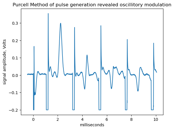
It was found that changes in \(\omega_1\) as small as \(10^4\) Hz would be significant enough to fully flip the sign of the spin echo equation modeled by Hahn. The variance in frequencies was eventually measured to be 12.3KHz, well within this range. Additionally, Hahn finds that the component of magnetization that is measured has an additional term: \(\cos(\Delta\omega t)\), where \(\Delta\omega = \omega_0 - \omega_1\), representing how off resonance the \(H_1\) field is. Thus, for certain errors in \(\omega_1\), an oscillatory modulation of the magnetization should be observed. Finally, Hahn also describes a scenario in which protons in the same molecule can have different Larmor frequencies due the shielding from their local electron densities, another possible cause of the modulated signal shown in Figure 3. The methods presented in this study, though unconventional in the field of pulsed NMR, are mostly robust to these effects, and may be desirable for experimentalists with lower quality set ups.
The physics set up used to collect spin echo signals consisted of an Alpha model 7500 electromagnet connected to an Alpha model 7500PS DC power supply and an AC line regulator. To get a signal, the current from the power supply was turned slowly up to around 2.7 Amps, after which it was allowed to cool for around an hour while the field stabilized. This electromagnet provided the large \(H_0\) field, while a small coil, capable of holding glass vials containing samples, provided the RF (radio frequency) \(H_1\) field. The pulses were generated using an Arduino, after which a frequency of 10 MHz was generated over the pulses by the RF transmitter, which was driven by a CTS MX0045 crystal clock oscillator. The signal was then sent through a tuning circuit before being sent to the coil to drive \(H_1\). Finally, the spin echo signals were picked up from the coil and fed into a Picoscope 2204A, where data was analyzed using the Picoscope T&M 7 software.

There are three variables that need to be optimized in order to see a maximal spin echo signal: the \(H_0\) field strength, and the 90 and 180 degree pulse times. Since the most sensitive of these is the \(H_0\) strength, this was varied first, over a small range on the order of tens of micro Amperes. The 90 and 180 times used for this step were estimated from the field strengths of \(H_0\) and \(H_1\), using the equation, \(t_\pi = \frac{H_0}{2H_1f}\), where f is the Larmor frequency. Though an accurate measurement of the \(H_1\) field could not be made, it was found to be at the largest \(10^{-4}\) T, which would place the optimal pulse lengths at around 50 and 100 \(\mu\)s for the \(90\degree\) and \(180\degree\) pulse lengths, respectively. To more accurately optimize the pulse times, two methods were developed. First, the times were simply randomly searched through to optimize the spin echo. Second, a spin echo was actually observed after the application of a 180-90 pulse sequence. As there is no \(180\degree\) pulse to re-cluster the spins in the x-y plane, with correct pulse times this echo should be impossible. Thus, it was assumed that this was due to imperfect pulse times, providing a simple way to optimize the pulse times: by elimination of this spin echo. Complete elimination of this spin echo proved impossible, though, likely due to timing inconsistencies in the set up.
Next, the magnetic moment of the proton was estimated from a sample of glycerin. As implied by Equation 2, the frequency of the RF \(H_1\) pulse that eliminates the z component of the effective field will actually be the Larmor frequency, \(\omega_0 = \gamma H_0\). Thus, simply measuring the frequency of the \(H_1\) pulse is enough to determine the proton moment. To do this, the input signal was transformed using the Picoscope software, from which a frequency and approximate measure of standard deviation was calculated.
The measurement of the three time constants were performed by taking traces of spin echo experiments with the Picoscope. For the measurement of \(T_2^*\) in glycerin, an average over 500 waveforms was used to get a nice spin echo signal, from which a full width half max was extracted using python, and used to calculate \(T_2^*\). Likewise, for \(T_1\), a large number of traces were averaged together, while keeping tau constant at 1.5ms. The variable altered between experiments was the time between different 90-180 sequences. For each time between sequences, T, the maximum value of the averaged spin echo peak was extracted.
Estimates of \(T_2\) suffered greatly from the oscillatory modulation of the echo signal. To measure \(T_2\), the time between \(90\degree\) and \(180\degree\) pulses, \(\tau\), was varied and the maximum value of the spin echo at \(2\tau\) was recorded. Since the effect of the modulation was worse for larger tau, some materials had to be manually analyzed. Instead of looking at the average waveform, many waveforms were extracted. If the peak in the region of the absolute value of the spin echo was larger than a threshold of 0.2V (above the noise level), it was kept and averaged.
For estimations of \(T_1\) and \(T_2\), Python was utilized to extract the maximum value of each averaged waveform. The log of this maximum was then plotted versus the two timescales varied, from which a linear or cubic fit was created using linear regression. The uncertainty in the estimate was extracted from the error in the estimate of the slope from the linear regression, which was given systematic errors corresponding to the noise of the system, \(\pm 0.097V\), as an input. Due to time limitations, only one curve could be collected per sample.
First, the magnetic moment of the proton was calculated. As mentioned, a measurement of the \(\omega_1\) driving \(H_1\) suffices to determine the Larmor frequency. From the Larmor frequency, we can determine the proton moment using the equations \(\mu_p = \gamma \frac{\hbar}{2}\), and \(\gamma = \frac{2\pi f}{H_0}\). The frequency of \(H_1\) was determined to be 10.00 MHz \(\pm\) 12.3KHz by using the fast Fourier transform algorithm from the numpy package to extract a peak in frequency. The error was estimated from the full width half max of the peak. From this estimation, the proton moment was estimated to be \(\mu_p = 1.416e-26 \pm 1.74e-29\) J/T, within 0.4% of the accepted value of \(1.4106e-26\) J/T.
Next, \(T_2^*\) was calculated for glycerin. Choosing a constant \(\tau = 2.0\)ms for each pulse sequence, \(T_2^*\) was calculated from the variance of a gaussian fitted to the spin echo curve, the functional form of which is predicted by Equation 4.
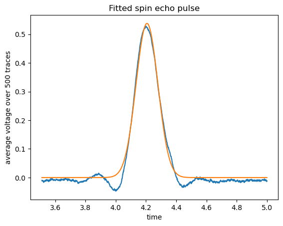

From this gaussian, \(T_2^*\) was estimated to be 72.2 \(\pm\) 1.8 \(\mu\)s. Despite the low \(\tau\) used in this run, it is worth noting the slight modulation at the edges of the gaussian, which may effectively be shrinking the width of the gaussian, meaning the value presented here may be an underestimate.
Next, \(T_1\) was estimated for glycerin, water, and the four concentrations of Copper Sulfate by varying the time, T, between spin echo experiments. Figure 5a shows the spin echo amplitude for varying T, for glycerin and water. The values of \(T_1\) calculated for each material are summarized in Table 1. The exponential plots qualitatively confirm the exponential relationship of longitudinal relaxation presented in Equation 3. Further, the difference in relaxation times between glycerin and water reveals the strong effect of viscosity on spin coherence. For higher viscosity materials, at a given temperature, the molecules will have more rotational energy than translational, simply due to the constraints from the high viscosity. It can be shown that the relaxation rate \(T_1\) is minimized when the frequency of the molecules rotation matches the Larmor frequency. As viscosity increases, the molecular "tumbling" becomes more energetic, and this condition gets closer to being satisfied, effectively decreasing \(T_1\) with viscosity\(^{[4]}\). The \(T_1\) times for the various Copper Sulfate concentrations likewise reveal the clear relationship between relaxation times and the presence of paramagnetic ions. Copper ions, containing unpaired electrons, will alter the local magnetic field due to the field produced by the magnetic moment of the unpaired electron. These electron moments will be oriented randomly due to thermal effects and molecular motion. This alteration of the local field is enough to strongly perturb the field around the two proton containing hydrogen atoms in water, causing the proton’s spins collective motion to de-phase. Thus, for higher Copper Sulfate concentration, the \(T_1\) relaxation time would decrease, as observed\(^{[5]}\).
Finally, \(T_2\) was measured for all of the liquids, minus water. The maximum spin echo magnitude versus time between \(90\degree\) and \(180\degree\) pulses is plotted for glycerin and the \(10^{17}\) ions/mL Copper Sulfate solution in Figure 5b. Much of the discussion on viscosity and ion concentration applies to \(T_2\) trends, as the de-cohering effects for bulk magnetization presented here will cause disruption along all axis, whether in the x-y plane or not. One important effect was the inclusion of the self diffusion constant, k, that was necessary for to fit the data for the lowest Copper Sulfate concentrations. For compounds with lower self diffusion, like glycerin, this effect could be ignored, as Hahn did in his original 1950 work. When self diffusion was sufficiently present, the log of the maximum amplitudes was fit to a cubic function rather than a linear one. The final calculated values are summarized in Table 1.
| \(T_1\) | \(T_2\) | |
|---|---|---|
| Glycerin | 42.2 \(\pm\) 2.0 ms | 22.7 \(\pm\) 2.32 ms |
| Water | 2.9 \(\pm\) 1.1 s | —— |
| 17 | 2.0 \(\pm\) 0.62 s | 70.6 \(\pm\) 5.8 ms |
| 18 | 0.52 \(\pm\) 0.65 s | 44.2 \(\pm\) 13.8 ms |
| 19 | 26.2 \(\pm\) 9.0 ms | 13.5 \(\pm\) 1.9 ms |
| 20 | 2.2 \(\pm\) 3.5 ms | 0.81 \(\pm\) 0.19 ms |
In conclusion, despite high noise levels in the data collected, we were able to develop methods to extract relaxation constants mostly robust against noise. Through the course of this experiment, the magnetic moment of the proton was determined from the driving frequency of the \(H_1\) field to be \(\mu_p = 1.416e-26 \pm 1.74e-29\) J/T, within 0.4% of the accepted value. Further, to our knowledge, accurate estimate of the relaxation times of glycerin were recorded, along with measurements of water and Copper Sulfate from \(10^{17}\) to \(10^{20}\) ions/mL. The dependence of the relaxation times on viscosity and dissolved ion concentration was also found, from trends in the relaxation times between glycerin and the rest of the samples, and the different Copper Sulfate concentrations. In future iterations of the study, we plan to further study the effect of viscosity on relaxation times using epoxy resin, which should change its relaxation constants as it cures. Furthermore, we plan to investigate the cause of the oscillatory echo modulation observed, as it remained ambiguous.