June 2025 Note: I originally planned to include the Kane-Mele model in this paper, but ended up not having the time to write about it. Also I wasn't very happy with the explanations at the end of the paper. In the future I plan to come back here and edit this to add Kane-Mele and expand basically every part but I need to do some review first. Also, I checked and all of the figures are from the topcondmat school (which is great), and are available under a CC liscense.

Introduction

In the previous 30 years it have become increasingly clear that topology is a necessary tool for understanding condensed matter systems. An elegant example of a system exhibiting nontrivial topological effects without the addition of an external magnetic field is the Haldane model, first proposed by Duncan Haldane in 1988. This model showed that a two-dimensional crystal can exhibit a quantized Hall conductance, or the quantum anomalous Hall effect (QAH), purely due to the lattice geometry and local time-reversal symmetry breaking, rather than through an externally applied magnetic field.

The Haldane model itself is an elaboration on the tight binding model for a simple honeycomb lattice. It consists of the nearest-neighbor (NN) real hopping term, present in the original model, and a next-nearest-neighbor (NNN) complex hopping. The complex phase added on mimics the effect of a staggered magnetic field that has no net flux per unit cell. This breaks time-reversal symmetry locally, but preserves translational symmetry. Importantly, this leads to a band structure that is gapped at the K and K’ points of the lattice, unlike in the original model. But, for certain values of the NNN hopping term, and another added mass-like term, the gap can actually be closed, causing a band inversion. It is at band inversions like these that topologically interesting phenomena occurs, and in this case, it gives rise to a Berry phase which implies a nonzero Chern number. The presence of this nontrivial topology manifests itself in edge states that give rise to a quantized Hall conductivity \(\sigma_{AH} = C\frac{e^2}{h}\), where C is the integer valued Chern number. The Haldane model serves as an important theoretical model for understanding the calculations of Berry curvature, Chern numbers, and bulk-boundary correspondence.

To this day, the Haldane model remains an important model in the field of condensed matter. The model laid the groundwork for making experimental predictions about Chern insulators, and provided the tools necessary for later models, such as the Kane-Mele model, which investigated the addition of spin to the Haldane model, and was the basis for the prediction of the quantum spin Hall effect. Numerous computer programs have additionally been developed for the model, due to the difficulty of doing many of the calculations without severe approximation.

The Haldane Model

As mentioned, the Haldane model was the first model to explicitly derive a mechanism for the quantum anomalous hall effect (QAH). The key insight into recovering the QAH effect was the introduction of a next-nearest-neighbor (NNN) hopping term into the Hamiltonian, which in this case was defined on a honeycomb lattice. First, we review the Hamiltonian and band structure of the honeycomb lattice, which will give us insights into how the Haldane model operates.

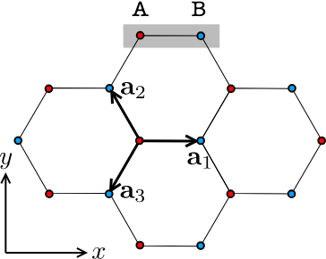
The honeycomb lattice is first defined with the following vectors:

\[\vec{a_1} = (1,0)\] \[\vec{a_2} = (-\frac{1}{2},\frac{\sqrt{3}}{2})\] \[\vec{a_3} = (-\frac{1}{2},-\frac{\sqrt{3}}{2})\]

The vectors \(\vec{a_i}\) represent the lattice basis vectors, while the vectors \(\vec{\delta_i}\) represent the displacement vectors from an atom in sub lattice A from all three nearest neighbors in sub lattice B, and vice versa. We can additionally get the Bravais lattice vectors of the system, which can be used to define the K and K’ points, \(K = (\frac{2\pi}{3},\frac{2\pi}{3\sqrt{3}})\) and \(K' = (\frac{2\pi}{3},-\frac{2\pi}{3\sqrt{3}})\). The most elegant way to solve this problem is done in the following way. We can define the total wavefunction in momentum space as the sum of the momentum space wavefunction for sub lattices A and B, where N is the total number of unit cells in the crystal.

\[\ket{\psi_k} = \alpha\ket{A_k} + \beta\ket{B_k}\]

\[\ket{A_k} = \frac{1}{\sqrt{N}}\sum_{\vec{R}}e^{i\vec{k}\cdot\vec{R}}\ket{A_{\vec{R}}}\] \[\ket{B_k} = \frac{1}{\sqrt{N}}\sum_{\vec{R}}e^{i\vec{k}\cdot\vec{R}}\ket{B_{\vec{R}}}\]

We further assume that the onsite energy of every A and B atom is zero, meaning that: \(\braket{A_R | \hat{H} | A_R} = 0\), and likewise for atoms in the B sub lattice. We introduce the nearest neighbor hopping term \(t_1\) as the following...

\[\braket{A_{\vec{R}+\vec{\delta_i}} | \hat{H} | B_{\vec{R}}} = -t_1\]

and likewise for the opposite combination of states. This statement essentially expresses that there is a non-zero overlap in energy between the nearest neighbor lattice sites. We are interested in the Hamiltonian in momentum space, so we can solve for it using the state expressed in this space. \[\begin{aligned} \braket{A_k | \hat{H} | B_k} = \frac{1}{N}\sum_{\vec{R},\vec{R'}}e^{i\vec{k}(\vec{R}-\vec{R'})}\\\times\braket{A_{\vec{R'}} | \hat{H} | B_{\vec{R}}} \end{aligned}\]

\[= \frac{1}{N}\sum_{\vec{R},\vec{R'}}e^{i\vec{k}(\vec{R}-\vec{R'})}(-t_1)(\delta_{\vec{R'}-(\vec{R} + \vec{\delta_i})})\] \[=\frac{1}{N}\sum_{\vec{R}}(-t_1)(e^{i\vec{k}\cdot\vec{\delta_i}})\] \[=-t_1f(k)\]

Where in the second and third steps there is an implied sum over all of the delta basis vectors, and the final complex function is simply written as \(f(k)\). We can similarly show that expectation values taken between states on the same lattice will be zero. This is because of the \(\bra{A_{R'}}\hat{H}\ket{A_R} = 0\) term which will appear in the sum, that will always be zero no matter the displacement between neighboring A atoms, and likewise for atoms on the B sub lattice.

The Hamiltonian of the system can then be written in matrix form: \[\begin{aligned} H(\vec{k}) = \begin{pmatrix} 0 & -t_1f(k) \\ -t_1f^*(k) & 0 \end{pmatrix} \end{aligned}\]

Diagonalizing this Hamiltonian, we get an energy relation, which is captured in the famous band diagram:

In the Haldane model, two more terms are introduced. First, a term to introduce a difference in energy between the A sub lattice and the B sub lattice, M. Second, the next-nearest-neighbor (NNN) hopping effect is introduced, with strength \(t_2\). The Hamiltonian is given below in the second quantized notation [2].

\[\begin{aligned} H = M \sum_i (-1)^{\tau_i} c_i^\dagger c_i + t_1 \sum_{\langle i,j \rangle} (c_i^\dagger c_j + h.c.) \\ + t_2 \sum_{\langle\langle i,j \rangle\rangle} (ic_i^\dagger c_j + h.c.) \end{aligned}\]

Here, the \(c_i\) operators represent the fermionic creation and annihilation operators at all sites, numbered through i and j. The variable \(\tau_i\) is simply either one or two depending on which sub lattice is being described. Finally, the NNN term describes how the wavefunction picks up a phase of +i as it hops between next nearest neighbors in the forward direction. In the original Haldane model paper this term was left as some ambiguous phase \(e^{i\phi}\), but here the simpler case is treated. Importantly, this term breaks time reversal symmetry (TRS), as complex conjugation would flip the sign of the i in the NNN term. This Hamiltonian can be written in the same form as for the normal honeycomb lattice:

\[\begin{aligned} H(\vec{k}) = h_0(\vec{k}) + M\sigma^z + 2t_2\sum_i\sigma^z\sin(\vec{k}\cdot\vec{d}) \end{aligned}\]

Where the new set of vectors \(d_i\) have been introduced to represent the distances between nearest neighbors of the same sub lattice A or B. Since the important topological effects will happen around Dirac cones in the band structure at the K and K’ points, the Hamiltonian is expanded about these points as \(\vec{k} = \vec{K} + \vec{q}\). Considering q negligible in the sin term...

\[\begin{aligned} H(\vec{k}) = \begin{pmatrix} M + 3\sqrt{3}t_2 & -t_1f(\vec{K} + \vec{q}) \\ -t_1f^*(\vec{K} + \vec{q}) & -M - 3\sqrt{3}t_2 \end{pmatrix} \end{aligned}\]

The off diagonal terms of the matrix are intentionally left un-simplified as at the K and K’ points these will go to zero. The important physics occurs due to the diagonal terms. The total energy for the valence and conduction bands will thus be:

\[E_K = \pm (M + 3\sqrt{3}t_2)\]

Thus, the band structure of the Haldane model is essentially the same as for the simple graphene model presented before, but with a band gap at the K and K’ points caused by the new terms introduced. For the K’ point the relation is essentially the same apart from the \(t_2\) term acquiring a minus sign. The important feature of this Hamiltonian is what happens when \(t_2\) is varied such that the energy flips sign. When the energy flips sign, the lower energy term of the Hamiltonian (already diagonalized in the sub lattice A and B basis), or the lower band, will be entirely localized on one of the sub lattices. Because of the different energies at the K and K’ points, it is possible that the valence band could be localized on A at one of these points, but at B at the other. This character of the valence band does require a band inversion, or a case where the band gap energy goes to zero.

In principle, we can now calculate the Chern number, which will reveal the importance of the topology of the band structure. To do this, we can note that the Berry curvature around the K and K’ points approaches a delta function as the band gap closes for changing \(t_2\). Due to this fact, we can simply calculate the Berry curvature from the Hamiltonian we expanded about these two points, as this approximation should capture almost all of the curvature. To do this, we can diagonalize the Hamiltonian given earlier, and extract eigenstates \(\ket{u_-}\) and \(\ket{u_+}\), corresponding to the states in the valence and conduction bands. The Berry curvature then becomes [2]:

\[\omega^-(k) = \partial_{k_x}\bra{u_-}\partial_{k_y}\ket{u_-} - \partial_{k_y}\bra{u_-}\partial_{k_x}\ket{u_-}\]

We can show that for some small region \(\Lambda = |\vec{q}|\) this equals:

\[\omega^-(k) = \frac{M + 3\sqrt{3}t_2}{2((M + 3\sqrt{3}t_2)^2 + q_x^2+q_y^2)^{3/2}}\]

At this point we can integrate to get the Chern number of the lower band as a function of the sign of the energy term. Here we note that, since almost all of the Brillioun zone will have zero curvature, the integral is taken in the only approximately non-zero region of \(\Lambda\).

\[C = \frac{1}{2\pi}\int_{BZ}d^2k(\omega^-(k))\] \[C = \pi sign(M + 3\sqrt{3}t_2)\]

This result will be true up to some correction due to the delata function approximation. To get the full Chern number, we have to add up the contributions of the K and K’ points. For different values of M and \(t_2\), the results of the Chern number integral at K and K’ will either sum or cancel. There exist two regions in this parameter space where the Chern number is nonzero.

The nonzero Chern number found here is important in that it gives rise to the quantum anomalous Hall effect. This result can be formally proven with linear response theory, as in [2], however, the result is stated here:

\[\sigma_{AH} = C\frac{e^2}{h}\]

The bulk properties of the insulator are able to generate edge modes that generate the responses required for this Hall effect. The basis of these edge modes stems from single crossings of states from the valence bands to the conduction bands, and vice versa [1].

Conclusion

In conclusion, the Haldane model was shown to exhibit interesting topological properties, which give rise to the quantum anamolous Hall effect. To build up this model, a regular model of graphene was first employed and solved, which was shown to have no band gap whatsoever. Then, after introducing a site dependent energy, M, and a next-nearest-neighbor hopping term that broke time reversal symmetry, the Haldane model was shown to exhibit a changing Chern number based on the varying of these parameters. In the much simplified case of being near band inversion, where the Berry curvature was assumed to be localized almost entirely at the K and K’ points, in what are essentially delta functions, the Chern number was solved for by integrating the calculated Berry Curvature over a small region deemed to sufficiently capture the Berry curvature. Using this method, we were able to recapture the \(Z_1\) index that describes the topology of this band structure. This topology is important in that it gives rise to dissipation less edge states, described by band crossings. Another model that took Haldane’s model one step further was the Kane-Mele model, which introduced electron spins into the Hamiltonian. Importantly, this model found that the two spin states could essentially be described as decoupled; that the model could be thought of as two Haldane models with opposite spin, giving rise to the idea of the Kane-Mele model having a \(Z_2\) topological index. This model was able to provide a theoretical prediction of the quantum spin Hall effect. In future papers, we plane to explore this model more.